StudyZin: Your Ultimate Q&A Repository
StudyZin has more than one million of the most reliable questions to enable any student earn good understanding of their subjects. In case an answer seems to be difficult, Zin AI takes it a step farther as it dissects the problem and provides detailed step-by-step explanation, while also incorporating visuals such as diagrams and pictures for effective communication. StudyZin has also been noted to have certain similarities with Chegg and CourseHero in the sense that it is designed to provide academic assistance, only this time it has many advantages over those two services, including being able to make learning easier, faster, cheaper and more enjoyable through the use of interactive explanations and supporting inclusion.
Zin AI: Your Intelligent Study Companion
Zin AI is a little more than just a study tool. It is a complete learning partner. With the help of the feedback from its intelligent insights and the ai in real time, Zin AI makes you domineer. It integrates the aspects of both classical education with modern technologies. It transforms the all boring studying part into something that is creative, aggressive, and fun making you discover new heights and soon improving visibility.
Unleash the Power of AI in Learning
Zin AI employs new technology like artificial intelligence while maintaining a personalized approach to the learning process. Therefore, education becomes better and easier. This AI enabled platform suits your personal learning requirements, enabling you to gain a solid knowledge of difficult subjects in no time. Use Free ChatGPT and get Free textbook Answers.
Advanced Student Help Website
As the education landscape evolves, so do the tools available to students. A modern student-help website utilizes advanced AI technologies like ChatGPT to offer comprehensive and innovative solutions for learners. Below are the main features of our website, each designed to simplify students' academic journeys while harnessing the power of artificial intelligence.
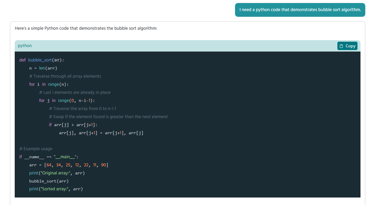
Instant Answers: Step-by-Step Explanations
The Instant Answers feature is crafted to deliver precise and reliable solutions to students' academic questions. It employs cutting-edge AI that analyzes a query and provides step-by-step explanations, ensuring students not only receive the correct answer but also comprehend the process behind it.
- Solves complex mathematical problems.
- Offers clear explanations for scientific concepts.
- Answers questions related to literature, history, or general knowledge.
Why It’s Unique: Unlike traditional search engines, this feature delves into the reasoning and logic, aiding students in grasping concepts and enhancing critical thinking. By promoting understanding rather than rote memorization, this feature empowers learners to master challenging topics independently.
Image Attachment: Assignment and Quiz Support
The Image Attachment feature enables users to upload images, such as assignments, handwritten notes, or quiz problems. The AI processes the image, extracts relevant data, and provides instant feedback, answers, or solutions.
- Scanning and solving handwritten math problems.
- Decoding text from blurry or poorly written notes.
- Interpreting diagrams, equations, or images from quiz questions.
Technological Highlight: Utilizing Optical Character Recognition (OCR) integrated with AI like ChatGPT, this feature ensures that even challenging, non-standard text or visual information is processed accurately. For students facing difficulties with handwritten or image-based questions, this feature bridges the gap between traditional and digital learning.
Voice Input: Hands-Free Assistance
Voice input provides an easy way for students to engage with the platform. By speaking into their device, users can ask questions, dictate assignments, or clarify doubts without the need to type.
- Quicker interactions, especially while multitasking.
- Accessibility for individuals with typing challenges or disabilities.
- Enhanced pronunciation and language skills as the AI offers feedback on voice-to-text conversion.
Technology at Play: This feature utilizes natural language processing (NLP) and voice recognition technology, resulting in a smooth and intuitive user experience. Voice input streamlines the process for students who are busy or prefer to communicate verbally, making it an essential tool for effortless learning.
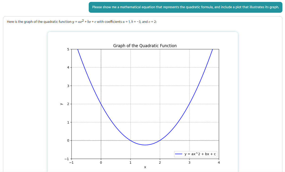
Graph/Plots Generation: Visualizing Data and Equations
The Graph/Plots Generation feature is perfect for visual learners who need to interpret data or grasp mathematical equations through graphs. By inputting data sets or equations, students can produce clear, customizable visual representations.
- Plotting linear, quadratic, or trigonometric equations.
- Visualizing statistical data for projects or presentations.
- Analyzing trends in scientific experiments.
Why It Matters: Visualization enhances understanding. A graph that accompanies a mathematical explanation helps students grasp concepts more effectively and derive meaningful insights. This feature ensures that students not only perform calculations but also interpret results, which is a vital skill in STEM disciplines.
Create Images: AI-Generated
The Create Images feature enables users to produce high-quality, AI-driven images for various applications. Whether for academic projects, presentations, or personal creativity, students can specify their needs and receive tailored visuals in just seconds.
- Generating educational diagrams such as flowcharts, mind maps, or concept illustrations.
- Creating visuals for digital storytelling or creative assignments.
- Producing engaging graphics for social media or personal branding.
AI Advantage: Utilizing advanced image-generation models, this tool provides visually appealing and contextually relevant images with minimal user effort. This feature not only sparks creativity but also saves time, helping students excel in their presentations and assignments.
PowerPoint/ Google Slides: Coming Soon
The forthcoming PowerPoint Slides feature is set to transform how students craft presentations. With AI-generated templates, layouts, and content suggestions, this tool will allow users to create professional, visually striking slides quickly.
- Pre-designed templates customized for various academic fields.
- Automatic generation of slide content from written notes or outlines.
- Smart formatting and alignment for a polished appearance.
Future Potential: This feature will merge productivity with aesthetics, ensuring students can deliver impactful presentations with less effort. By automating slide creation, it will boost efficiency, giving students more time to concentrate on their research and analysis.
How AI Transforms Education
These features leverage the latest advancements in AI, ensuring they are accurate, user-friendly, and adaptable. Here’s how AI is changing these tools:
- Personalized Learning: The platform tailors itself to each student’s preferred learning style, whether they learn best through visual aids, hands-on activities, or listening to explanations.
- Efficiency: Automation streamlines repetitive tasks like creating graphs or slides, saving valuable time.
- Inclusivity: Voice recognition and image processing enhance accessibility for a broader range of learners, including those with disabilities.
- Real-Time Feedback: Immediate responses and visual aids enable students to spot and correct errors on the spot, speeding up their learning process.
Zin AI at a Glance